Support Vector Machines (SVMs)

Geometry, Convex Optimization, Duality, Kernel Methods, and Extensions to SVC and SVR.

Notation

• Vectors

$x_i \in \mathbb{R}^d$ — input (feature) vector of the $i$-th data point

$w \in \mathbb{R}^d$ — normal vector to the separating hyperplane

$\phi(x) \in \mathcal{H}$ — feature-space representation of input $x$

• Scalars

$y_i={−1,+1}$ — class label of the $i$-th data point

$b \in \mathbb{R}$ — bias (offset) term of the hyperplane

$\gamma \in \mathbb{R}_+$ — geometric margin

$\xi_i \in \mathbb{R}_+$ — slack variable

$C \in \mathbb{R}_+$ — regularization parameter

$\epsilon \in \mathbb{R}_+$ — SVR tube radius

• Dual Variables (Scalars)

$\alpha_i \ge 0$ — Lagrange multipliers (classification)

$\alpha_i^{\ast} \ge 0$ — Lagrange multipliers (SVR)

$\mu_i \ge 0$ — Lagrange multipliers for slack constraints

• Functions and Operators

$f(x)=\operatorname{sign}(\langle w,x \rangle + b)$ — decision function

$\mathcal{K}(x,z)$ — kernel function

⟨⋅,⋅⟩ — Euclidean inner product

$\left\lVert \ast \right\rVert_2$ — Euclidean norm

• Sets and Indices

$n$ — number of training samples

$d$ — dimension of the input space

$i,j$ — data point indices

• Optimal Quantities

$w^{\ast}, b^{\ast}$ — optimal primal solution

$\alpha^{\ast}$ — optimal dual variables

1. The Classification(Binary) Problem as Geometry

We begin with the binary classification problem from a purely geometric perspective. Let the training set be

${(x_i, y_i)}_{i=1}^n$, where $x_i \in \mathbb{R}^d$ and $y_i \in {-1, +1}$.

The goal is to construct a decision rule that separates points of different labels with maximal robustness(maximize the minimum distance from a data point to our hyperplane, that gives = simpler model = better generalization). SVMs approach this problem by explicitly reasoning about geometry in the input space, rather than by introducing a loss function from the outset.

1.1. Linear Separability and Hyperplanes

A hyperplane in $\mathbb{R}^d$ is defined as the set

where $w \in \mathbb{R}^d$ is the normal vector to the hyperplane and $b \in \mathbb{R}$ is the bias term

We are building a model for a classification problem(let it be binary) .The hyperplane induces a classifier of the form

small definition

The space is partitioned into two half-spaces:

$ \langle w, x \rangle + b > 0$ and $ \langle w, x \rangle + b < 0$,

which correspond to the two class labels ${-1,+1}$

Linear Separability

The dataset is said to be linearly separable if there exists at least one pair $(w,b)$ such that

for all

Proof:

the correct predictions are defined as : $y_i = 1 <=> \langle w,x \rangle + b \ge 0$ and

$y_i = -1 <=> \langle w,x \rangle + b < 0 $ thus, if we multiply LHS and RHS , we get

\(y_i(\langle w,x \rangle + b) > 0\)

This condition guarantees that a hyperplane exists which correctly classifies all training points.

At this stage, infinitely many separating hyperplanes may exist.But the central question becomes :

• Which separating hyperplane should be chosen?

And tadaa SVMs answer this by introducing the notion of margin!!

1.2. Functional and Geometric Margins

Functional Margin

Given a classifier $(w,b)$, the functional margin of a labeled point $(x_i,y_i)$ is defined as

The functional margin of the dataset is

While convenient algebraically, the functional margin depends on the scale of $w$ and $b$. Multiplying $(w,b)$ by any positive constant scales the functional margin arbitrarily, without changing the decision boundary.

This makes the functional margin unsuitable as a geometric notion of confidence.

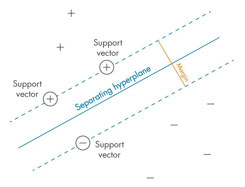
Geometric Margin

The geometric margin is the distance between the hyperplane(decision boundary) and the support vectors(closest data points to the hyperplane).

source

The distance from a point $x$ to the hyperplane $H$ is

Proof:

let’s assume we have an arbitrary point $x_0$ and a hyperplane defined by the equation $\langle w, x \rangle + b = 0$ . We need to find the perpendicular distance $d$ from $x_{0}$ to this hyperplane

Consider any point $x_{p}$ on the hyperplane which is the projection of $x_0$ onto that plane. The vector from $x_{p}$ to $x_{0}$ , i.e. , $(x_{0} - x_{p})$ is parallel to the normal vector of the hyperplane $w$ . Thus, the distance $d$ is the length of the vector $(x_{0} - x_{p})$ . The projection of the vector $(x_{0} - x_{p})$ onto the unit normal vector ( $\frac{w}{\left\lVert w \right\rVert}_{2} $ ) will give us the desired distance $d$ :

Since point $x_{p}$ lies on the hyperplane, its coordinates satisfy the equation

or

Let’s expand the dot product in the distance formula:

Substitute $\langle w, x_{p} \rangle = -b$ :

Accordingly, the geometric margin of a labeled point $(x_{i},y_{i})$ is

The geometric margin of the dataset is

Unlike the functional margin, the geometric margin is invariant under rescaling of $(w,b)$ and has a direct geometric interpretation.

1.3. Margin Maximization Principle

Among all separating hyperplanes, Support Vector Machines choose the one that maximizes the geometric margin :

Geometrically, this corresponds to selecting the hyperplane that is as far as possible from the closest data points of either class.

Why Margin Matters ?

Maximizing the margin has several fundamental consequences:

1. Robustness to perturbations

   A larger margin implies that small perturbations of the input vectors are less likely to change the classification outcome.

2. Capacity control

   From statistical learning theory, classifiers with larger margins have lower effective capacity, leading to better generalization guarantees.

3. Uniqueness of solution

   While many separating hyperplanes may exist, the maximum-margin hyperplane is unique (up to translation of $b$) under mild conditions.

This principle provides the conceptual bridge between geometry and generalization, which will later be formalized through convex optimization and duality.

1.4. Scale Normalization

Because the decision boundary defined by $(w,b)$ is invariant under positive rescaling, we may impose a normalization constraint without loss of generality as $\hat{\gamma_i} = 1$ . Which means

Proof :

We can always find some $(w,b)$ such that $\min\lvert \langle w,x \rangle + b \rvert = 1$

Let $\min( \langle w,x \rangle + b) = c$

Thus, if we substitue $w,b$ with $w_\text{new} = \frac{w}{c}$ and $b_\text{new} = \frac{b}{c}$ we get

Now let’s maximize the margin keeping in mind those derivations

Under this normalization, maximizing the geometric margin is equivalent to minimizing $\left\lVert w \right\rVert_{2}$.

This observation leads directly to the primal optimization formulation of the hard-margin SVM.

2. Hard-Margin Support Vector Machine

2.1. Primal Optimization Problem

Under the normalization constraint, the problem of finding the maximum-margin separating hyperplane can be written as the following optimization problem:

$\min_{w,b} \frac{1}{2} \left\lVert w \right\rVert_2^2$ s.t. $y_i(\langle w, x_i \rangle + b) \ge 1,$ $i = 1,2,…,n.$

This is known as the hard-margin Support Vector Machine. The fraction $\frac{1}{2}$ and a term $\left\lVert w \right\rVert_{2}^{2}$ are added for mathematical convenience(for smoothness and differentiability when optimizing) . Minimizing $\left\lVert w \right\rVert_{2} $ is equivalent to minimizing $\left\lVert w \right\rVert_{2}^{2}$ cause it yields the same optimal result.

Remarks

1. Quadratic objective

   The objective function $\frac{1}{2} \left\lVert w \right\rVert_2^2$ is a strictly convex quadratic function in $w$.

2. Linear Constraints

   The constraints are affine functions of $(w,b)$, defining a convex feasible region.

3. Convexity

   Since the objective is convex and the feasible set is convex, this is a convex optimization problem. Any local minimum is also a global minimum.

4. Uniqueness

   The solution for $w$ is unique whenever the data are linearly separable. The bias term $b$ may not be unique though.

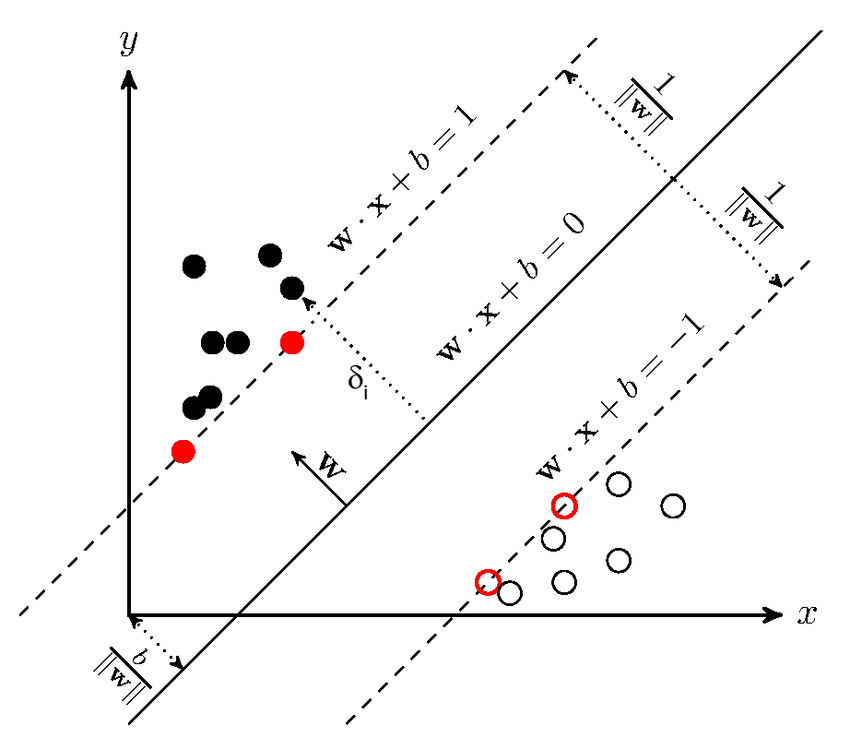
2.2. Geometric Interpretation of the Constraints

Each constraint

enforces that the point $x_i$ lies on the correct side of the hyperplane and at least a distance $\frac{1}{\left\lVert w \right\rVert_2}$ from it.

The points that satisfy

lie exactly on the margin boundaries. These points are the support vectors. All other points satisfy the constraints strictly and do not influence the optimal solution.

2.3. Support Vectors and Sparsity

A fundamental consequence of the margin maximization formulation is that only a subset of the training points determines the solution!!

Definition.

A data point $(x_i,y_i)$ is called a support vector if

where $(w^{\ast},b^{\ast})$ denotes the optimal solution of the primal problem.

source

Geometrically, support vectors are the points closest to the decision boundary. Removing any non-support vector does not change the optimal hyperplane.

This sparsity property will later emerge naturally from the DUAL formulation.

You may ask “Why the Primal Formulation Is Not Enough?”

While the primal problem provides clear geometric intuition, it has two important limitations:

1.It relies explicitly on the assumption of linear separability.

2.It depends directly on the inner product $\langle w, x \rangle$ , which restricts us to linear decision boundaries. Both limitations will be addressed by:

• Introducing Lagrangian duality

• Reformulating the problem in terms of inner products between data points.

To expose the structure of the solution and prepare the ground for kernel methods, we now derive the dual formulation of the hard-margin Support Vector Machine using Lagrangian duality and the Karush–Kuhn–Tucker conditions.

3. Lagrangian Duality and The Dual Problem

The primal formulation of the hard-margin Support Vector Machine is a convex optimization problem with inequality constraints. To analyze its structure and derive a more flexible representation, we apply Lagrangian duality. Before we start, let me firstly introduce several concepts.

* — WHAT IS A CONVEX OPTIMIZATION PROBLEM? —

A constrained optimization problem is called a convex optimization problem if

$\min_x{f(x)}$ <- $f(x)$ is a convex funciton

s.t.

$g_i(x)\le 0$ for all $i = 1,…,m$ <- $g_i(x)$ is also a convex function

and $ h_j(x)=0$ for all $j=1,…,n$ <- $h_j(x)=0$ is an affine equality (thus, a convex set)

For any optimization problem we apply KKT conditions,which are necessary but for most cases NOT sufficient . HOWEVER! a special case arise when we deal with a convex constrained optimization problem , KKT conditions are still necessary AND become sufficient as they fully characterize the solution.

* — Karush-Kuhn-Tucker(KKT) Conditions —

1. Primal Feasibility

The solution must satisfy the constraints :

1. Dual Feasibility

Lagrange multipliers must satisfy

1. Stationarity

Gradient of the Lagrangian with respect to primal variables is zero :

Stationarity connects primal variables to dual variables

1. Complementary Slackness

For each component, either the constraint is active or its multiplier is zero, never both nonzero :

3.1. The Primal Optimization Problem, The Lagrangian

We introduce a non-negative Lagrange multiplier $\alpha_i \ge 0$ for each constraint

The Lagrangian associated with the primal problem is

where $\alpha = (\alpha_1,…,\alpha_n)$ - vector of lagrange multipliers

The primal problem corresponds to minimizing $\mathcal{L}$ with respect to $(w,b)$ and maximizing with respect to $\alpha \ge 0$

To obtain the dual formulation, we minimize the Lagrangian with respect to the primal variables $w$ and $b$

Let’s compute the derivatives with respect to primal variables and apply stationarity conditions

Derivative with respect to $w$

Setting the derivative to zero yiels

This equation already reveals an important fact : the normal vector $w$ lies in the span of the training points

Derivative with respect to $b$

Setting it to zero gives

3.2. The Dual Optimization Problem

Substituting the stationarity conditions back into the Lagrangian eliminates the primal variables $(w,b)$. The resulting dual objective depends only on the dual variables $\alpha_i$.

Usually it’s convinient to maximize the dual while minimizing the primal so let’s simplify and derive the dual problem. Firstly,we expand our primal lagrangian(hard margin)

Now let’s substitute the derivatives w.r.t. primal variables

Keep in mind that

Thus,

Our Dual

The dual optimization problem becomes

subject to

This is a quadratic programming problem in the variables $\alpha_i$

Remarks

1.Dependence on inner products only

The data appear exclusively through inner products $\langle x_i,x_j \rangle$. This observation is the key to kernel methods.

2.Dimensionality

The optimization is performed in $\mathbb{R}^n$, independent of the ambient dimension $d$.

3.Convexity

The dual objective is concave, and the feasible region is convex. Therefore, the dual problem has a unique global maximum.

3.3. Connecting the dual

Using the stationarity condition for $w$, the classifier can be written as

Only points with $\alpha_i > 0$ contribute to the sum , yielding a sparse representation.

The dual formulation reveals that the Support Vector Machine depends on the data only through inner products. This observation allows the extension of SVMs to nonlinear decision boundaries via kernel methods.

4. Kernel Methods: From Inner Products to Nonlinear Decision Boundaries

4.1. From Featute Maps to Kernels

Suppose we map inputs into a (possibly high-dimensional) feature space:

source

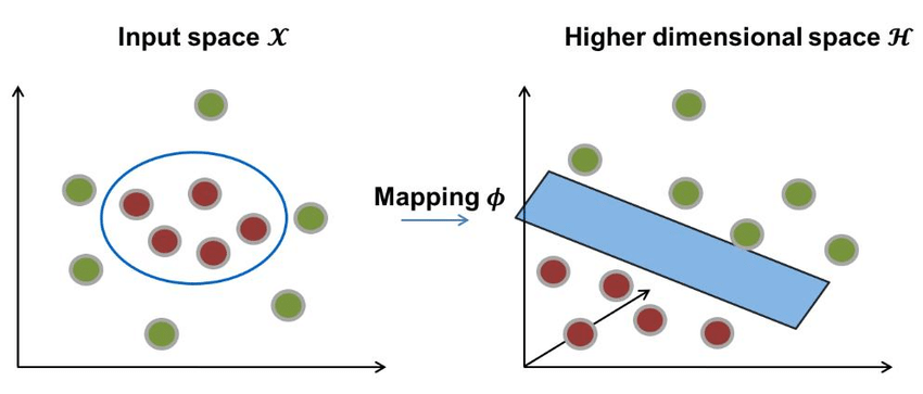
Where $\mathcal{H}$ is a Hilbert space(Inner-product space) . A linear classifier in feature space has the form

If we try to directly work with the feature mapping $\phi(x)$ , we may need to handle extremely high-dimensional vectors. The kernel method avoids explicit computation of those mappings.

4.2. Kernel Trick

Let’s firstly introduce the concept of a kernel

— * What is a kernel K ? —

A kernel is a function

such that

for some feature mapping $\phi$ into some inner-product space $\mathcal{H}$

In the SVM dual , we replace every $\langle x_i,x_j \rangle$ by $\mathcal{K}(x_i,x_j)$.Thee hard-margin dual becomes:

subject to

The corresponding decision function is

Only support vectors (those with $\alpha_i > 0$) contribute to the sum.

4.3. Which Functions Are Valid Kernels?

Not every symmetric function $\mathcal{K}(x,z)$ is a valid kernel. The key requirement is that the kernel corresponds to an inner product in some (possibly infinite-dimensional) feature space. Let me formalize it by introducing the definition of the Gram matrix and a simple version of Mercer’s Theorem.

Definition

Given points $x_1,…,x_n$, we define the Gram matrix $G \in \mathbb{R}^{n \times n}$ by

A function $\mathcal{K}$ is a valid (Mercer) kernel if, for any finite set ${x_1,…,x_n}$, the Gram matrix $G$ is positive semidefinite (PSD), i.e.

or $c^{\intercal} Gc \ge 0 $ for all $c \in \mathbb{R}^n$. This PSD condition is what ensures that $\mathcal{K}$ behaves like an inner product.

In general ,a Gram matrix $G$ of vectors $x_1,x_2,…,x_n$ is the matrix of all possible dot products of those vectors :

Mercer’s Theorem in a nutshell

If $\mathcal{K}$ is symmetric and positive semidefinite (under mild regularity assumptions), then there exists a feature mapping $\phi$ into a Hilbert space $\mathcal{H}$ such that

Thus,using $\mathcal{K}$ in the dual is just the same as running a linear SVM in the feature space $\mathcal{H}$, without explicitly knowing the mapping $\phi$.

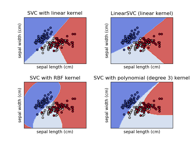
4.4. Examples of Most Common Kernels

1.Linear Kernel

2.Polynomial Kernel

$c \ge 0, p \in \mathbb{N}$.

3.Gaussian(RBF) kernel

$\sigma > 0$.

source

The kernalized dual allows creating nonlinear decision boundaries, however it still assumes perfect separability in feature space. In practice , that ideal separability is RARELY achieved , thus let me now tell you about slack variables and the soft-margin SVM.

5. Soft-Margin Support Vector Machines

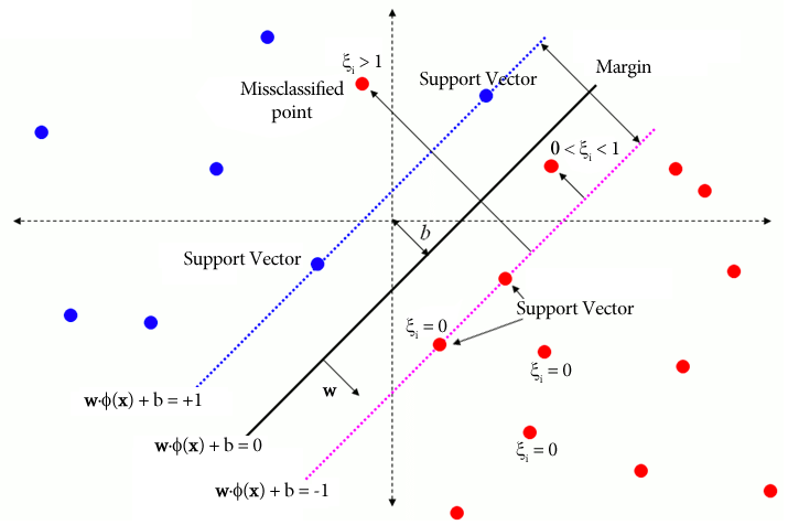
5.1. Slack Variables and Constraint Relaxation

For each training point , we introduce a slack variable $\xi_i \ge 0$ that measures the degree of constraint violation. The margin constraints become

Interpretation of $\xi_i$ :

• $\xi_i = 0$ : point lies on or outside the margin and correctly classified.
• $0 < \xi_i < 1$ : point is correctly classified but violates the margin.
• $\xi_i \ge 1$ : point is misclassified.

source

5.2. Primal Soft-Margin Optimization Problem

The soft-margin SVM trades off margin maximization against constraint violations:

subject to

$i = 1,…,n$ and $\xi_i \ge 0$

Here the hyperparameter $C > 0$ controls the bias-variance tradeoff like :

• Large C : heavy penalty to violations = low bias, high variance
• Small C : allows violations for wider margin = higher bias , lower variance

Now, before we continue ,I will show you another, BUT FOUNDATIONAL concept for SVMs - the hinge loss

Definition

5.3. Connection to Hinge Loss

The constrained soft-margin problem can be rewritten as an unconstrained regularized risk minimization problem.Then the soft-margin SVM is equivalent to:

This makes explicit the connection between SVMs and empirical risk minimization(ERM), while preserving a geometric interpretation via the margin.

5.4. Dual Formulation of the Soft-Margin SVM

Following the same procedure as for the hard-margin but we introduce another lagrange multiplier $\mu_i \ge 0$ for $\xi_i \ge 0$, let’s derive it :

I’ve already introduced the primal problem , now let’s construct the primal lagrangian :

stationarity w.r.t. primal variables

thus, $ C - \alpha_i -\mu_i = 0 $ => $\mu_i = C - \alpha_i$

And from knowing that $\mu_i \ge 0$ : $ C - \alpha_i \ge 0 $ => $\alpha_i \le C$ => $0 \le \alpha_i \le C$

$w = \sum_i\alpha_ix_iy_i$

$\sum_i\alpha_iy_i = 0$

Substituting into primal yields the dual

And finally the dual optimization problem :

subject to

Compared to the hard-margin case, the dual variables are now box-constrained.

5.5. Decision Function ( Kernalized)

The final classifier has the form

The bias term 𝑏 b can be computed using any support vector with $0 \le \alpha_i \le C$.

The soft-margin formulation provides robustness to noise while preserving convexity and sparsity. We now extend the same principles to regression, leading to Support Vector Regression.

6. Support Vector Regression (SVR)

Support Vector Regression extends the maximum-margin principle to real-valued outputs by introducing an ε-insensitive loss. Instead of separating classes, SVR seeks a function that approximates the data while remaining as flat as possible.

6.1. Regression as Function Approximation

Given training data

We consider linear predictors of the form

As in classification, flatness is measured by the norm $\left\lVert w\right\rVert_2^2 $. SVR therefore minimizes $\left\lVert w\right\rVert_2^2 $ subject to an _error tolerance*

6.2. $\epsilon$-Insensitive Tube

SVR introduces a tube of radius $\epsilon > 0$ around the regression function

Errors inside this tube are ignored(only deviations $> \epsilon$ are penalized) which gives a better robustness to outliers.

We also include 2 slack variables to allow violations :

• $\xi_i \ge 0$ for points above the tube
• $\xi_i^{\ast} \ge 0$ for points below the tube

The constraints become :

source

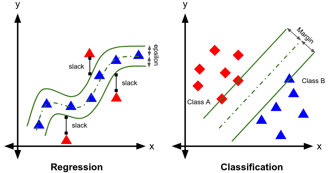
6.3. Primal Optimization Problem for SVR

The $\epsilon$-SVR primal problemmm is:

subject to :

Same as in classification :

• C controls the penalty for deviations outside the tube. *The problem is still convex

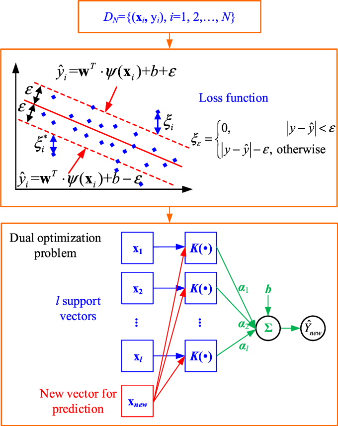
$\epsilon$-Insensitive Loss

The primal problem is equivalent to minimizing a regularized empirical risk with $\epsilon$-insensitive loss:

Thus:

6.4. Dual Formulation of SVR

Introduce Lagrange multipliers :

• $\alpha_i,\alpha_i^{\ast} \ge 0$ for the $\epsilon$-tube constraints,

• $\mu_i,\mu_i^{\ast} \ge 0$ for non-negativity of slack variables.

After minimizing the primal Lagrangian w.r.t. $w$ and $b$ , the dual problem becomes:

subject to:

6.5. Decision Function (SVR)

The regression function is:

Only points with $\vert\alpha_i - \alpha_i^{\ast}\vert > 0$ conribute (these are the support vectors)

6.6. Geometrical Interpretation

• Points inside the $\epsilon$-tube : $\alpha_i = \alpha_i^{\ast} = 0$
• Points on the boundary of the tube(supp. vec-s): $0 < \alpha_i < C $ or $0 < \alpha_i^{\ast} < C$
• Points outside the tube : $\alpha_i = C$ or $\alpha_i^{\ast} = C$

Thus, as in SVC, SVR yields a sparse output.

source

Implementing SVM from scratch in Python(Soft-margin)

Requirements : Python(>2.7), NumPy, matplotlib, sklearn

Core algrorithm

#svm.py <-----
# !!!!
import numpy as np


class SVM:

   def __init__(self, C = 1.0):
      # C = hyperparameter for penalty
      self.C = C
      self.w = 0
      self.b = 0
   def hingeloss(self, w, b, x, y):
      # Regularization term (L_2)
      reg = 0.5 * (w * w)

      for i in range(x.shape[0]):
         # Optimization term
         opt_term = y[i] * ((np.dot(w, x[i])) + b)

         # calculating loss
         loss = reg + self.C * max(0, 1-opt_term)
      return loss[0][0]
   def fit(self, X, Y, batch_size=100, learning_rate=0.001, epochs=1000):

      number_of_features = X.shape[1]
      number_of_samples = X.shape[0]

      c = self.C

      # Creating ids from 0 to number_of_samples - 1
      ids = np.arange(number_of_samples)

      # Random shuffle of samples
      np.random.shuffle(ids)

      w = np.zeros((1, number_of_features))
      b = 0
      losses = []

      # Gradient Descent logic
      for i in range(epochs):
         # Calculating the Hinge Loss
         l = self.hingeloss(w, b, X, Y)
         losses.append(l)

         for batch_initial in range(0, number_of_samples, batch_size):
            grad_w = 0
            grad_b = 0

            for j in range(batch_initial, batch_initial + batch_size):
               if j < number_of_samples:
                  x = ids[j]
                  ti = Y[x] * (np.dot(w, X[x].T) + b)

                  if ti > 1:
                     grad_w += 0
                     grad_b += 0
                  else:
                     # Calculating the gradients
                     grad_w += c * Y[x] * X[x]
                     grad_b += c * Y[x]

            # Updating weights and bias
            w = w - learning_rate * w + learning_rate * grad_w
            b = b + learning_rate * grad_b

         self.w = w
         self.b = b

         return self.w, self.b, losses
   def predict(self, X):
      prediction = np.dot(X, self.w[0]) + self.b
      return np.sign(prediction)

You may be confused why we update w and b like that . But the reason is quite simple , let learning rate = $\eta$ and our cost function (objective func.)

Also let

that’s the loss per sample,

be the loss over the whole dataset. Taking the gradients with respect to $w$ and $b$ yields:

and

Also taking the gradients of hingeloss per sample w.r.t. $w$ and $b$ gives

and

Thus,

and

We defined negatives of those grads as grad_w and grad_b respectively. Remembering the grad descent update rule :

Substituting our variables of interest and their gradients gives us :

and

Now let’s create a random dataset(Binary classification)

import numpy as np
from sklearn.metrics import accuracy_score
from sklearn.model_selection import train_test_split

X, y = datasets.make_blobs(
      n_samples = 100,
      n_features = 2,
      centers = 2,
      cluster_std = 1,
      random_state=67
    )

# Cause binary classification
y = np.where(y == 0, -1, 1)
#Split
X_train, X_test, y_train, y_test = train_test_split(X, y, test_size=0.5, random_state=228)

Training our SVM

from svm import SVM
svm = SVM()
w, b, losses = svm.fit(X_train, y_train)

Producing the predictions and checking

preds = svm.predict(X_test)

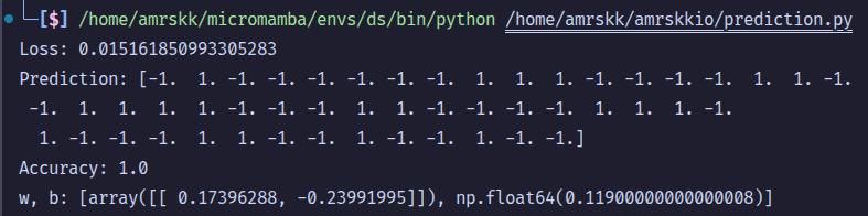
# Loss
err = losses.pop()

print("Loss:", err)
print("Prediction:", preds)
print("Accuracy:", accuracy_score(preds, y_test))
print("w, b:", [w, b])

Output[1] :

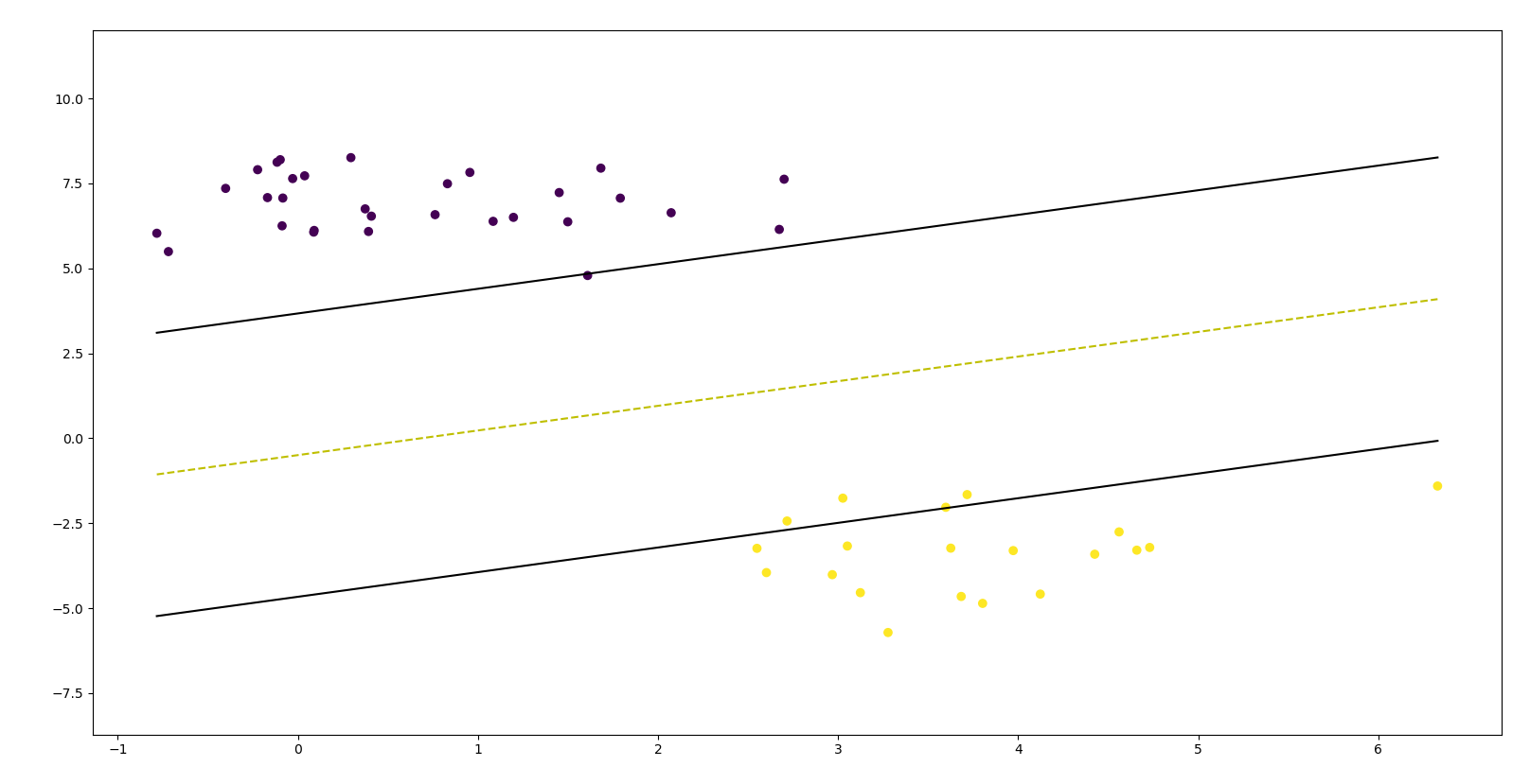
Visualizing SVM on the test set

import matplotlib.pyplot as plt
def visualize_svm():
   def get_hyperplane_value(x, w, b, offset):
      return (-w[0][0] * x + b + offset) / w[0][1]

   fig = plt.figure()
   ax = fig.add_subplot(1,1,1)
   plt.scatter(X_test[:, 0], X_test[:, 1], marker="o", c=y_test)

   x0_1 = np.amin(X_test[:, 0])
   x0_2 = np.amax(X_test[:, 0])

   x1_1 = get_hyperplane_value(x0_1, w, b, 0)
   x1_2 = get_hyperplane_value(x0_2, w, b, 0)

   x1_1_m = get_hyperplane_value(x0_1, w, b, -1)
   x1_2_m = get_hyperplane_value(x0_2, w, b, -1)

   x1_1_p = get_hyperplane_value(x0_1, w, b, 1)
   x1_2_p = get_hyperplane_value(x0_2, w, b, 1)

   ax.plot([x0_1, x0_2], [x1_1, x1_2], "y--")
   ax.plot([x0_1, x0_2], [x1_1_m, x1_2_m], "k")
   ax.plot([x0_1, x0_2], [x1_1_p, x1_2_p], "k")

   x1_min = np.amin(X[:, 1])
   x1_max = np.amax(X[:, 1])
   ax.set_ylim([x1_min - 3, x1_max + 3])

   plt.show()
visualize_svm()

Output[2] :

I hope this article would work for you as an assist to understand the SVM algorithm under the hood. Thank youuu for reading <3 !!